Risk-return tradeoff states that the potential return rises with an increase in risk. Using this principle, individuals associate low levels of uncertainty with low potential returns, and high levels of uncertainty or risk with high potential returns.
According to risk-return tradeoff, invested money can render higher profits only if the investor will accept a higher possibility of losses. When you invest, you make choices about what to do with your financial assets.
Risk is any uncertainty with respect to your investments that has the potential to negatively impact your financial welfare. For example, your investment value might rise or fall because of market conditions (market risk).
Return on investment (ROI) is an approximate measure of an investment’s profitability. ROI is calculated by subtracting the initial cost of the investment from its final value, then dividing this new number by the cost of the investment, and finally, multiplying it by 100.
Contents:
What is Risks and Returns?
In investing, risk and return are highly correlated. Increased potential returns on investment usually go hand-in-hand with increased risk. Different types of risks include project-specific risk, industry-specific risk, competitive risk, international risk, and market risk. Return refers to either gains or losses made from trading a security.
The return on an investment is expressed as a percentage and considered a random variable that takes any value within a given range. Several factors influence the type of returns that investors can expect from trading in the markets.
Diversification allows investors to reduce the overall risk associated with their portfolio but may limit potential returns. Making investments in only one market sector may, if that sector significantly outperforms the overall market, generate superior returns, but should the sector decline then you may experience lower returns than could have been achieved with a broadly diversified portfolio.
Risk is also defined in financial terms as the chance that an outcome or investment’s actual gains will differ from an expected outcome or return. Risk includes the possibility of losing some or all of an original investment.
Quantifiably, risk is usually assessed by considering historical behaviors and outcomes. In finance, standard deviation is a common metric associated with risk. Standard deviation provides a measure of the volatility of asset prices in comparison to their historical averages in a given time frame.
Overall, it is possible and prudent to manage investing risks by understanding the basics of risk and how it is measured. Learning the risks that can apply to different scenarios and some of the ways to manage them holistically will help all types of investors and business managers to avoid unnecessary and costly losses.
Risk and Return Examples
Let’s run through a few examples of risk and return.
Example:
Imagine there are two possible bonds you want to invest in: Bond X and Bond Z. And let’s say that Bond X has a 15% chance of non-payment and Bond X has a 45% chance of failure (loss). In the absence of any further data, you are of course more likely to select Bond A since it provides you with a higher chance of keeping your money. To thrive, Bond Z must boost its interest rates until the reward surpasses the danger of nonpayment. Bond Z can then entice you back despite its increased risk.
To compensate for the hazards, a riskier investment must provide higher profits. The gains are what attract some investors, while the danger deters others. A less risky investment, on the other hand, may provide relatively modest rates of return since the security of the investment is what brings investors in rather than the chance for higher returns.
Contents
Introduction
Present Value and Opportunity Cost of Capital
(a) Computing present value
(b) Present value and risk
Capital Budgeting
(a) Cost of capita
(b) An overview of capital budgeting
Measurement of Risk
(a) Definition of risk
(b) Quantification of risk
(c) Risk-free rate and risk premium
(d) Incorporation of risk in investment decisions
Measurement of Investment Returns
(a) Definition of investment
(b) Definition of return
(c) Calculation of return
(d) Returns on international investments
(e) Nominal and real returns
(f) Calculating expected rate of return
(g) Use of risks and returns in investment decisions
In Summary
Activity – Questions and Answers
Introduction
The impact of financial decisions can be measured by their net present value (NPV), which is the value created or destroyed by adopting a course of action. The concept of time value of money is important in gaining an understanding of how asset values are determined. It is therefore necessary for investors and investment advisers to understand this concept in determining the risk and return relationship of their investments. In this topic, we will introduce the concept of time value of money. We will also examine some capital budgeting techniques generally used in making project decisions.
Risk can be defined as the uncertainty of achieving the expected returns or the probability that the realised outcome will be different from the expected outcome. Investors would want to know about the riskiness of their investment and consider it in terms of the opportunity cost of capital. To do so, they must find a way to measure risk. There are several ways to measure risk. One way is to measure the variability of returns. However, this measurement may not be accurate in a portfolio context as movements between assets in a portfolio will result in diversification of risk.
This topic examines the measurement of risk for individual assets. We shall also be discussing the various methods of measuring returns.
Learning objectives
(a) Discuss the concept of time value of money and opportunity cost of capital;
(b) Examine the methods that can be used to make an investment decision; and
(c) Understand and illustrate the measurement of risk and return.
Present Value and Opportunity Cost of Capital
Computing present value
Before we enter into any discussion on risks and returns, it is useful to first revisit the concept of present value. Present value basically says that a ringgit today is worth more than a ringgit tomorrow because a ringgit invested today will earn interest and because of inflation.
Present value is simply computed by multiplying the future payoff by the discount factor. The discount factor is always less than 1 and is computed as follows:
Discount Factor = 1 / (1+r)
Where:
r = the reward that investors demand for accepting delayed payment
As a simple illustration, let us assume that you expect a payoff of RM50,000 at the end of the year. If the current fixed deposit interest rate for 1 year is 5%, how much would you have to place in the fixed deposit in order to have a payoff of RM50,000 at the end of the year? Simply multiply the discount factor with the future expected payoff as follows:
Present value,
= RM50,000 x 1 / (1 + 0.05)
= RM47,619.05
= RM47,620
The above shows that you would have to place RM47,620 in a fixed deposit that pays 5% interest per annum in order to have a payoff of RM50,000 at the end of the year.
Let us now assume that you have been asked to commit an investment of RM45,000 in an equity unit trust that promises a payoff of RM50,000 at the end of Year 1. You would be willing to pay a higher price of RM47,620 for this investment if your required rate of return is 5%. The market price, which is the same as the present value of investment, is computed by discounting the expected future payoffs by the rate of return offered by comparable alternatives. This rate of return is also known as the discount rate or the opportunity cost of capital as it represents returns foregone by investing in the unit trust rather than, say, placing it in the fixed deposit.
Present value and risk
The example set out in the above section contains an unrealistic assumption, i.e. the certainty of the payoff of RM50,000 from the equity unit trust investment. This RM50,000 payoff cannot be certain and at best represents a forecast of returns. As such, RM47,620 may not represent the current market value of the unit trust investment as investors can achieve a higher certainty of being paid RM50,000 at the end of the year by placing the same amount in the fixed deposit.
Most investors would like to avoid unnecessary risk without sacrificing return (i.e. a safe ringgit is worth more than a risky one).
Types of Risk and Return
There are several types of both risk and return.
Risks
Whenever you invest or save, there are different types of risks that can be involved. But there are typically two categories that the risks are placed into: systematic risks and unsystematic risks.
Systematic
Risks that can influence a complete economic market or at minimum a significant portion of it are known as systematic risks. They are the dangers of losing assets as a result of various macroeconomic or political risks which impact the general market performance. There are many types of systematic risks; a few of those are:
Political risk – Political risk arises largely as a result of political insecurity in a nation or area. For example, if a country goes to war, the firms that operate there are deemed unsafe, and therefore risky.
Market risk – Market risk is the byproduct of investors’ overall inclination to follow the market. So it is essentially the inclination of security values to shift together.
Exchange rate risk – This type of risk arises from the unpredictability of currency value fluctuations. As a result, it impacts enterprises that conduct foreign exchange operations, such as export and import firms, or firms that do business in a foreign country.
Interest rate risk – A shift in the market’s rate of interest causes this type of risk. It mostly affects fixed-income assets since bond costs are connected to interest rates, but it also affects the valuation of stocks.
Capital Budgeting Basics
Capital investments are long-term investments in which the assets involved have useful lives of multiple years. For example, constructing a new production facility and investing in machinery and equipment are capital investments. Capital budgeting is a method of estimating the financial viability of a capital investment over the life of the investment.
Unlike some other types of investment analysis, capital budgeting focuses on cash flows rather than profits. Capital budgeting involves identifying the cash in flows and cash out flows rather than accounting revenues and expenses flowing from the investment. For example, non-expense items like debt principal payments are included in capital budgeting because they are cash flow transactions. Conversely, non-cash expenses like depreciation are not included in capital budgeting (except to the extent they impact tax calculations for “after tax” cash flows) because they are not cash transactions. Instead, the cash flow expenditures associated with the actual purchase and/or financing of a capital asset are included in the analysis.
Capital Budgeting
Capital budgeting is the process of analysing projects for investment. A typical capital budgeting process can be summarised as follows:
(i) identify the set of available investment opportunities;
(ii) analyse each individual investment opportunity to estimate the future cash flows for each project under review and evaluate its profitability;
(iii) select the project that has the best fit with overall company strategies, taking into consideration the project timing and resources involved; and
(iv) monitor and post-auditing, which involve comparing actual results to the planned or projected results and explaining the differences to help improve future investment decision-making processes.
Capital budgeting involves the use of discounted cash flow analysis. To do this, the company would need to determine the appropriate discount rate. This would be based on the cost of capital. The cost of capital is the required rate of return for a capital budgeting project and is not the company’s historical cost of capital. In other words, the cost of capital is the return at which investors would provide financing for the capital budgeting project under consideration today.
Cost of capital
In general, the company’s capital components include debt, preference shares and common equity. If a company decides to increase its total assets, that increase would have to be funded by an increase in one or more of the capital components. The cost of capital would be the weighted average cost of the capital components. We shall briefly look at each of these capital components and their costs.
Cost of debt
The cost of debt is the cost of debt financing to a company when it issues a bond or takes up a bank loan. The after-tax cost of debt [k d (1 — t)] is used in computing the weighted average cost of capital. This is provided by the effective cost of new debt (kd) less tax savings due to the deductibility of interest (kdt).
After-tax cost of debt,
= effective interest rate – tax savings
= kd — kd(t)
= kd d (1 — t)
Note that the cost of debt is the cost of new debt and not of existing or old debt.
Example:
Company A is planning to raise new debt at an effective interest rate of 10% per annum. Company A’s corporate tax rate is 25%. What is Company A’s after-tax cost of debt?
kd (1 -t) = 10% (1 -0.25) = 7.5%
If the company uses leasing as a source of capital, the cost of these leases should be included in the cost of capital. The cost of this form of borrowing is similar to that of the company’s other long-term borrowing.
Cost of preference shares
A preference share is a perpetuity that pays preference dividends forever (assuming that preference shares are not redeemable, it will be a perpetuity security). The cost of preference shares (kp) is computed as follows:
kp = Dp / Pnet
Where:
Dp = preference dividends
Pnet = net issuing price after deducting issuing costs
The equation for valuing preference shares can be expressed as follows:
Pp = Dp / rp
Where:
Pp – price of preference shares
rp – required rate of return
The equation for the cost of preference shares is basically a rearrangement of the valuation equation. Note, however, that kp will be slightly higher than rp to compensate for issuing costs.
Example:
Assume that Company A has decided to issue preference shares t hat pay preference dividends per share of RM5. Company A sells the preference shares for RM50 per share. Assume also that Company A’s issuing cost is approximately 5% for issue of new shares. Compute Company C’s cost of preference shares.
kp = 5/ [50x(1 – 0.05)] = 10.53%
Cost of retained earnings
The cost of retained earnings, k„ is the rate of return that a company’s ordinary shareholders would require on retained earnings (required rate of return) or the opportunity cost of retained earnings. The cost of retained earnings can be estimated by using one of the following two approaches:
CAPM Approach
The capital asset pricing model (CAPM) will be discussed in Topic 6 of this module. Principally, the CAPM equation can be expressed as:
Ks = rf + ß(rm- rf)
Where:
Ks = required rate of return
rf = risk-free rate
rm = expected rate of return of the market
(ß = beta of the share (the share’s risk measure)
The difficulty with using CAPM is in estimating all the variables such as beta and the market risk premium (rm – rf).
Example:
Let’s look at Company A again. Suppose Company A has a beta of 0.9. The current risk-free rate is 6% and expected rate of return of the FBM KLCI is 12%. Using the expected return of the index as a proxy for the expected return of the market, compute the required rate of return for Company A’s retained earnings.
ks = 6% + 0.9 ( 12% – 6%) = 11.4%
Dividend yield plus growth rate approach
This approach assumes that dividends are expected to grow at a constant rate (g) and as such, the current price of a share is:
P = D1 / (ks – g)
as such,
ks = (D1 / P) +g
where:
D1 = next year’s dividend
Ks = investor’s required rate of return
g = constant growth rate
The main difficulty in using this approach is the need to estimate the growth rate. You can use growth rates either projected by the company, research analysts or based on the following equation:
g = (retention rate) (expected return on equity)
Example:
Company A expected to pay out dividends of RM1.20 per share. The share currently sells for RM30 per share. Company A expects to retain 50% of its earnings and its expected return on equity is 2%. Compute Company A’s cost of equity.
g = 0.5x 12% = 6%
ks = (1.2/30) + 6% = 10%
Cost of newly issued equity
The cost of common equity (ke) will be higher than the cost of retained earnings due to flotation costs. Expanding from the dividend discount model above, the cost of common equity can be expressed as follows:
ke = D1 / [P1(1 – f)] + g
Where:
f = percentage of flotation cost incurred in selling new stock (current share price – funds received by the company)/current share price)
Example:
Based on the example above, assume Company A’s flotation cost is 11%. Compute the cost of new equity for Company A.
ke = D1 / [P0(1 – f)] + g = 1.2 / [30(1 – 0.11)] + 6% = 10.49%
Note: the cost of equity is generally higher than the cost of retained earnings due to flotation cost. In the example above, if Company C is not able to earn 10.49% on a project that is financed by the ssuance of new equity, its growth rate of 6% will not be achieved, resulting in a drop in the price of the company’s shares. As such, issuance of new equity by itself is not dilutive but the inability of the company to earn its cost of equity will result in dilution of earnings.
Weighted average cost of capital (WACC)
The WACC is simply the average of all the company’s cost components weightedaccording to the proportion of each cost component and can be expressed as:
WACC = Wd [kd(1 – t)] + Wp (kp) + We (ke)
Where, Wd, Wp and We – are simply the weights used for debt, preference shares and equity respectively and are based on the company’s optimal capital structure. Such weights should be based on market values of the company’s securities.
Example:
Assume Company C has determined that its optimal capital structure is 30% debt, 20% preference shares and 50% equity. In addition, the costs of its capital components are:
kd (1 – t) = 7.5%
kp = 10.5%
ks = 10%
ke = 10.5%
The WACC, if all new equity funds come from retained earnings, is:
WACC,
= wd [kd (1-t)] + wp(kp) + w5(k5)
= (0.3)(7.5%) + (0.2) (10.5%) + (0.5)(10%)
= 9.35%
The WACC, if all new equity funds come from new issuance of equity, is:
WACC,
= wd [kd (1-t)] + w(k) + We(ke)
= (0.3)(7.5%) + (0.2)(10.5%) + (0.5)(10.5%)
= 9.6%
Factors that affect cost of capital
Generally, there are two groups of factors that would affect a company’s cost of capital. The first consists of factors that are beyond the control of the company and the second are factors that are within the control of the company.
(a) Factors outside the control of the company:
(i) level of interest rates; and
(ii) tax rates.
(b) Factors within the control of the company:
(i) capital structure of the company;
(ii) dividend policy of the company; and
(iii) investment policy (the riskiness of the investments of the company).
An overview of capital budgeting
Capital budgeting is essentially about financial decisions in relation to the investments in or the retirement of a particular business or project. For example, they may include decisions on:
(a) investments in a new service line;
(b) replacement of plant and machinery;
(c) discontinuation of a product line;
(d) increase in the production capacity of a product; or
(e) production of a product component in-house as opposed to subcontracting it to third parties.
Why is the capital budgeting decision important? If a wrong decision is made, the company would lose some flexibility by being “locked in” during the life of the investment. A company’s capital budgeting decision will also affect its strategic plan.
Projects being considered can either be mutually exclusive, which means that only one project can be accepted and the others under consideration will be rejected, or independent, which means the projects are unrelated to one another. In the following sections, we shall discuss the guidelines for capital budgeting and their use in making project decisions.
There are several commonly used methods in assessing capital investment decisions, namely:
• net present value (NPV);
• internal rate of return (IRR);
• modified IRR;
• payback period (PBP); and
• discounted PBP.
Net present value (NPV)
Net present value (NPV) measures the difference between what the asset is worth (the present value of its expected future cash flows) and its cost. NPV is an effective way of evaluating projects as it is based on discounted cash flows over the life of the project.
NPV is basically the amount of net cash generated by the project after repaying the initial investment cost. A positive NPV means that shareholder’s wealth has been increased because the asset is worth more than it costs and vice versa. The formula to compute NPV is:
NPV,
= Present Value of expected future cash flow – Cost
=
Where:
= sum or present value of expected future cash flows
Ci = future cash flow at period i
R = discount rate
Co = cash outflow at time period 0 (i.e. today)
The decision rule: for independent projects, if NPV is positive, accept the project. If NPV is negative, reject the project. For mutually exclusive projects, choose the project with a higher NPV, subject to the NPV being positive.
Example:
The cash flows for two projects under consideration, Project A and B, are set out as follows:
NPV(A) = (5,000) + 3,0001(1.12)+ 1,8001(1.12)2+ 1,000/(1.12)3 + 800/(1.12)4 = RM333.71
NPV(B )= (5,000) + 1,500/(1.12) + 1,800/(1.12)2 + 2,800/(1.12)3 +70O/(1.12) = RM212.08
If projects A and B are independent, accept both. If the projects are mutually exclusive, accept only project A.
Internal rate of return
The internal rate of return (IRR) is basically the rate of return that equates the present value of the project’s expected cash flows with the present value of the project’s costs.
In other words, IRR is the rate of return for which the NPV is zero. To calculate IRR, you can use the trial and error method (i.e. by guessing the IRR figure and replacing it into the equation until you get the right answer), linear interpolation or a financial calculator.
The decision rule: The company should first decide on its hurdle rate, which is the minimum rate of return it will accept for a project (i.e. the company’s cost of capital).
This rate is then compared with the IRR. If the IRR is higher than the hurdle rate, accept the project.
Example:
Based on the same example:
Solving for IRR using interpolation:
IRR = kp + {(k(N) – kp) x [NPVp/ (NPVp – NPV(N))[}
Where:
Kp = the discount rate that results in a positive NPV
K(N) = the discount rate that results in a negative NPV
NPVp = positive NPV based on kp
NPV(N) = negative NPV based on k(N)
Project A:
NPVA = 0 = (5,000) + 3,000/(1+1 RRA) + 1,800/(1+IRRA)2 + 1,000/(1+IRRA)3 + 800/(1+1 RRA)4
Guess 14% for kp,
NPVp = (5,000) + 3,000/(1.14) + 1,800/(1.14)2+ 1,000/(1.14)3+ 800/(1.14)4 = RM165.26
Guess 17% for kp(N),
NPV(N) = (5,000) + 3,000/(1.17) + 1,800/(1.17)2+ 1,000/(1.17)3+ 800/(1.17) = RM(69.68)
IRRA = 14% + [(17% – 14%) x (165.26/234.90 = 16.11%
Project B:
NPVB = 0 = (5,000) + 1,500/(1+IRRB) + 1,800/(1+IRRB)2 + 2,800/(1+IRRB)3 + 700/(1+IRRB)4
Guess 12% for kp,
NPVp = (5,000) + 1,500/(1.12) + 1,800/(1.12)2+ 2,800/(1.12)3+ 700/(1.12)4 = RM212.08
Guess 15% for k(N),
NPV(N) = (5,000) + 1,500/(1.15) + 1,800/(1.15)2 + 2,800/(1.15)3 + 700/(1.15) = RM(93.32)
IRRB = 12% + [(15% – 12%) x (212.08/305.40)] = 14.08%
Note that when solving for IRR using linear interpolation, it is important to use NPVs that are as close to zero as possible. The larger the gap between the positive and negative NPVs selected, the higher will be the degree of inaccuracy.
Solving for IRRA (using a financial calculator) = 16.08%
Solving for IRRB (using a financial calculator) = 14.05%
Project A will be ranked above project B. Based on a hurdle rate of 12%, if both projects are independent, accept both. If they are mutually exclusive, accept only project A.
One weakness of IRR is that it assumes reinvestment of cash flows at the IRR rate. In addition; a project with non-normal cash flows (for example cash outflows during its life or at the end of its life) may have multiple IRRs. We shall demonstrate an example with multiple IRRs.
Example:
Compute the IRR of project K which has the following cash flows:
Using the trial and error method, we guess an IRR figure and replace it into the following equation:
4,000 = 25,000/(1 + IRR) + (25,000)/(i + IRR)2
Let’s arbitrarily try 10%;
4,000 = 25,000/1.1 + (25,000)/1.12
4,000 = 2,066.11
Next we try 25%:
4,000 = 25,000/1.25 + (25,000)/1.252 = 4,000
If we try a discount rate of 400%, we will find that it will also provide the same answer:
4,000 = 25,000/5 + (25,000)/52 = 4,000
Based on the above, project K has two IRRs, 25% and 400%. This is due to the double change in the sign of the cash flow stream. There can be as many different IRRs for as many changes in the sign of the cash flows. When this happens, the IRR method is not appropriate for the evaluation of investments or projects and the investor should then make the investment decision based on NPV or the modified IRR.
Modified IRR
The modified IRR (MIRR) is basically the internal rate of return for a series of periodic cash flows which considers both the cost of investment (or financing rate) and interest on reinvestment of cash. As demonstrated above, when there are positive and negative cash flows in the cash flow stream of a project, there is potential for more than one IRR.
In determining the MIRR, negative cash flows are financed at the financing rate and as such, are discounted at the financing rate (f-rate). Positive cash flows are reinvested at the reinvestment rate that reflects the return on an investment with a comparable risk (r-rate).
Generally, in determining the MIRR, the following steps could be used:
(i) Calculate the present value of negative cash flows at the f-rate.
(ii) Calculate the future value of positive cash flows at the r-rate.
(iii) Find the discount rate (the MIRR) which will equate the sum of the positive cash flows (the future value) with the sum of the negative cash flows (present value).
Example:
Assume project A and B have the following cash flows. The r-rate and f-rate for both projects are 12% and 10% respectively.
Remember: Negative cash flows are discounted to the present value at the f-rate and positive cash flows are reinvested at the r-rate to determine the future value.
To obtain MIRR,
Or by using a financial calculator:
The MIRR was designed to address the problems of IRR. This is because the MIRR incorporates a better reinvestment and financing rate assumption (recall that IRR assumes that cash flows are reinvested at IRR while the MIRR assumes that cash flows are reinvested at the investors’ required rate of return) and it avoids the multiple IRR problem.
Payback period (PIP)
PBP is the number of years required to recover the original cost of investment and the payback is based on cash flow. It is a measure of payback and not a measure of profitability.
PBP = Years before full recovery + (Unrecovered cost at the end of the year before full recovery / Cash flow in the following year)
The decision rule: An investment with a shorter payback period is preferred over one with a longer payback period. In deciding which project to accept and whether to accept a project or not, the company should compare the payback period with its own benchmark PBP.
The main drawback of using PBP is that it ignores the time value of money. It also fails to consider cash flows after the payback period and risk differences between projects.
In addition, the determination of the company’s benchmark PBP is too arbitrary.
Notwithstanding this, the PBP method is appealing as it is easy to compute and simple to understand. Because of its focus on cash flows before the payback period, PBP provides a form of control on liquidity and it serves as an indicator of project liquidity.
For example, a project with a 2-year payback may be more liquid than another project with 5-year payback.
Example:
Based on the same example:
In order to find the PBP for each project, determine the cumulative net cash flow of the projects which are set out in the following table:
PBPA = 2 + (200/1,000) = 2.20 years
PBPB = 2 + (1,700/2,800) = 2.61 years
Assume the company requires a payback period of 2.5 years (the benchmark payback period), then the company would accept only project A. If the company has a payback period of 3 years, then:
– if projects A and B are mutually exclusive, the company will accept project A only; and
– if projects A and B are independent, the company will accept both projects.
Discounted payback period (discounted POP)
As mentioned above, the PBP fails to consider the time value of money. The discounted PBP is an improvement on the PBP measure as it discounts the estimated cash flows by the project’s cost of capital.
The decision rule: an investment with shorter discounted PBP is preferred over one with a longer discounted PBP. Accept projects with discounted PBPs that are less than the company’s benchmark discounted PBP.
While the discounted PBP method incorporates time value of money into its analysis, it still fails to consider cash flows after the payback period. Discounted PBP is superior to the PBP method but not as conceptually correct as NPV.
Example:
Using the same example, assume that the company’s cost of capital is 12%.
Discounted PBPA = 3 + 174/508 = 3.34 years
Discounted PBPB = 3 + 233/445 = 3.52 years
If the company’s benchmark PBP is 4 years, accept both projects if they are independent and accept only project A if they are mutually exclusive.
Summary
NPV is a direct measure of the ringgit benefit of the project and it measures the amount of net cash generated by the project after repaying the initial investment cost.
The IRR is the rate of return that equates the present value of the project’s cash flows with the initial investment costs. The IRR measures profitability as a percentage of return and provides safety margin information on the project. The IRR basically tells you how much returns on a project can fall before the company’s capital is at risk.
Generally, when comparing IRR and NPV, NPV is considered to be a better measure because it assumes that the reinvestment rate of cash flows is the cost of capital while IRR assumes the reinvestment rate to be at IRR. In addition, the problem of multiple IRRs does not exist with the NPV method.
The MIRR is the internal rate of return for a series of periodic cash flows, considering both the cost of investment (financing cost) and interest on reinvestment of cash. The MIRR is considered an improvement to IRR in that it incorporates the reinvestment rate and financing rate for the cash flow streams of the project.
The PBP and discounted PBP methods basically compute the number of years before recovery of the original cost of investment. These methods result in an indicator of risk and liquidity of a project. The shorter the payback, the higher the liquidity of the project and the lower the risk (i.e. cash flows are expected earlier in the project life).
However, the PBP method ignores the time value of money. Furthermore, the PBP and discounted PBP methods do not consider cash flows after the payback period.
Measurement of Risk
Definition of risk
Risk can be defined as the uncertainty of future outcomes or the probability of an adverse outcome. If we invest in a project and expect a 15% return per annum on the investment, the risk involved is the chance of not achieving the 15% return. Investors are, in general, risk averse and therefore would avoid unnecessary risk. If investors have to assume more risk than they prefer, the rewards have to be large enough to compensate for the extra risk. The reward for taking risk is called the risk premium.
When investors assume risk for high returns, they are said to speculate. When they assume risk without a reasonable prospect of gain, they are said to gamble.
One method of defining risk is based on the portfolio theory and the capital market theory by Harry Markowitz (which will be discussed in greater detail under Topic 6).
Basically, the portfolio theory states that, under a specified set of assumptions, all rational, profit-maximising investors want to hold a completely diversified market portfolio of risky assets and they would borrow or lend to arrive at a risk level that is consistent with their risk preferences. Based on this, total portfolio risk can be decomposed into systematic and non-systematic risk.
Systematic risk (market or non-diversifiable risk) is the measurement of the co-movement of an asset with the market portfolio. Systematic risk measures common sources of return variation that cannot be diversified away. As systematic risk cannot be diversified away, the market compensates investors for this risk. Systematic risk can refer to macro events in the economy that might hinder the achievement of targeted expected returns such as changes in inflation, interest rates and government policies.
Market risks are beyond the direct control of the company and affect all economic entities in the market, although each entity might be affected to a different degree. In making an investment decision, rational investors would incorporate the expected changes in these market variables and impute them in the required rate of return for the investment. However, the possibility of unexpected changes to these forecasts represents an additional source of risk. For example, if a 9% interest rate was forecast and incorporated in an investment, a source of market risk on the investment is if the actual interest rate for that period increases to 12% (or 3%).
Non-systematic risk (unique, specific or diversifiable risk) is the measurement of the variance of the individual assets/companies that is not related to the market portfolio but is due to the unique features of the assets/companies. For example, management problems, production problems, logistic problems or labour problems are sources of specific risk. This component of risk is assumed to be diversifiable, i.e. can be eliminated through diversification. This is based on the notion that if more than one company is incorporated in a portfolio, the weaknesses of each company will be compensated (and diversified) by the strengths of other companies.
Investors need to incorporate their estimates of risk in the investment decision. Before this can be done, they need to quantify the total, market and specific risks of the investment. Since only market risk is compensated in the market, the quantification of this risk would allow investors to identify investments with different levels of market risk and decide if the investments offer a commensurate level of rewards, given the level of the investors’ risk aversion.
What is Investment Decision?
Investment decision refers to financial resource allocation. Investors opt for the most suitable assets or investment opportunities based on risk profiles, investment objectives, and return expectations.
The term investment strategy refers to a set of principles designed to help an individual investor achieve their financial and investment goals. This plan is what guides an investor’s decisions based on goals, risk tolerance, and future needs for capital.1 They can vary from conservative (where they follow a low-risk strategy where the focus is on wealth protection) while others are highly aggressive (seeking rapid growth by focusing on capital appreciation).2
Fidelity. “Investment Strategy,” Page 3. Accessed March 31, 2021.
Investors can use their strategies to formulate their own portfolios or do so through a financial professional. Strategies aren’t static, which means they need to be reviewed periodically as circumstances change.
Quantification of risk
One measure of risk is the variance of returns. The variance of returns (or the standard deviation which is computed as the square-root of the variance of returns) measures the dispersion of returns around the expected return from the investment. The greater the variance, the higher the dispersion of returns around the expected return, the smaller the chance of actually achieving the expected return and, therefore, the higher the risk.
In general, the variance (a2) or standard deviation (a) of returns on an investment can be computed based on the following formulas:
ex-post basis:
Or on ex-ante basis:
Where:
σ2 = variance of returns
R1 = returns on the investment
E(r) = average or the mean returns
n = number of returns
P1 = probability of generating that particular return
The following example demonstrates the computation of the variance of returns and of standard deviation:
Based on a 68% confidence level (in which the returns will fall between +/- 1 standard deviation from the mean) and the standard deviation of 2.94%, the returns on this investment are expected to range from 8.06% (11 % – 2.94%) to 13.94% (11 % + 2.94). What does a 68% confidence level mean? Based on statistical principles, assuming a normal distribution of returns for an investment, a normal curve can be wholly described by its mean and standard deviation. In a normal curve, 68% of returns would fall between +/- 1 standard deviation of the mean, 99% of returns would fall within +/- 2.5 standard deviation of the mean and 99.99% of returns would fall within +/- 4 standard deviation of the mean (these numbers can be established from the Z-statistic tables found in statistic textbooks).
A standard deviation of 2.94% is considered a small deviation and hence the investment has lower risk compared to investments that have, for example, a standard deviation of 10%. In this case, if the average return on this investment is also 11 %, then the dispersion of possible returns (based on a 68% confidence level) would be between 1% (11 % – 10%) and 21% (11% + 10%). Holding all things constant, the wider the dispersion of returns, the riskier the investment.
Coefficient of variation
The usage of variances and standard deviations as measures of risk may be misleading (as we shall demonstrate below). The coefficient of variation (CV) is a relative measure of variability to indicate risk per unit of expected return and is computed based on the following formula:
CV = Standard deviation of returns/expected rate of return
Assuming an investor is considering two investments, stocks A and B, with the following expected returns and standard deviations:
CVA = 7%/10% = 0.7
CVB = 5%/6% = 0.83
Using absolute measures of risk, stock A with a standard deviation of 7% would appear to be riskier than stock B, with a standard deviation of 5%.
However, stock A has a CV of 0.7 while stock B has a CV of 0.83. This shows that stock A has less risk per unit of return.
Risk-free rate and risk premium
The risk-free rate (rf) is the basic interest rate that an investor would demand for a risk-free investment. The real rf assumes an inflation-free economy. The nominal rf is the risk-free rate after adjusting for inflation. From the real risk-free rate, an investor’s required rate of return on a risk-free investment can be computed as follows:
Nominal, rf = (1 + Real rf)(1 + Expected rate inflation) – 1
A risk-free investment is one in which both the amount and timing of cash flow is known with certainty. Most investments are not risk-free in nature. As such, investors would require rates of return that are higher than the nominal risk-free rate to compensate them for that uncertainty. This additional required rate of return is called a risk premium.
The risk premium is a function of several fundamental sources of risk. Business risk is the uncertainty of income flows caused by the nature of the company’s business.
Financial risk arises from the method of financing undertaken by the company for its investments and operations. Liquidity risk is the uncertainty about the time and price an asset can be converted into cash in the secondary market. For international investors, the risk premium would also include exchange rate risk and country risk.
Incorporation of risk in investment decisions
In evaluating investments and making investment decisions, investors (and financial managers) need to be concerned about the timing and uncertainty of future cash flows and their effects. Based on NPV, future expected cash flows are discounted to the present value and the sum of these discounted cash flows are then compared to the sum of the initial investment. Only projects with the sum of present value of cash flows exceeding the initial investment (in other words, when NPV is positive) are considered for potential investment.
One of the methods used to account for risk is to incorporate the risk factor of the investment into the rate used to discount future cash flows (the risk-adjusted discount rate). For projects with higher risk, higher discount rates are used and vice versa. The rationale is that investors are assumed to be risk averse and thus would require a higher rate of return (which is the discount rate) on risky investments and vice versa.
This way, investors can make an investment decision by comparing the risk-adjusted required rate of return of the investment with the expected rate of return. If the risk adjusted rate of return is higher than the expected rate of return, the investor would reject the investment and vice versa.
Another method for an investor to evaluate an investment is using the certainty equivalent method. The method enables the investor to compare the value of different investments with different levels of risk. Based on the assumption that investors are generally risk averse, an investor would choose an investment with a lower level of risk for a certain level of return or a higher level of return for a certain level of risk. Let’s illustrate the certainty equivalent method by looking at an example.
Example:
Assume investor A is considering two investments. One of them is a risk-free government security with a par value of RM1,000. The current risk-free rate (the yield on the risk free investment) is 6%. The other investment is a corporate bond with a 1-year promised return of RM1,200 (including coupon).
In evaluating the alternative opportunities, investor A should first determine the present value of the risk-free investment as follows:
Present value risk free = 1,000/1.06 = RM943.40
In order to determine the risk-adjusted rate of return (the required return for risky investments), Investor A should compute the discount rate that equates the present value of the risk-free investment with the future value of the risky investment as follows:
943.40 = 1,200/(1 + r) = 27.2%
This means that the investor would require a return of 27.2% for the risky investment in order to be equivalent to the risk-free investment.
Note that the certainty equivalent method is suitable when the investor knows exactly what risk-return trade-offs he or she is willing to make. Otherwise, the risk-adjusted discount rate would be a more appropriate way of comparing investments.
Measurement of Investment Returns
Definition of investment
An investment can be defined as a current commitment of money for a certain period of time to derive future receipts that will compensate the investor for:
(a) the time value of funds committed;
(b) the expected inflation rate; and
(c) the uncertainty (risk) of future receipts.
These future receipts are the investor’s required rate of return.
Definition of return
Returns are rewards for undertaking an investment. To put it differently, returns are gains normally expected from deferring current consumption of income. Risk-averse investors seek to maximise returns per unit of risk on their investments and do so by comparing alternative investments based on this criteria. There are three different types of rates of return, namely:
(i) Required rate of return
The required rate of return is the minimum return that an investor must earn to be willing to make an investment. One way to derive this rate of return is by looking at alternative investments of equal risk and the investor’s opportunity cost.
(ii) Expected rate of return
The expected rate of return is the rate of return an investor would expect from the investment given its level of risk. Put it differently, it is the rate of return that would equate the NPV to zero (when NPV is zero, the investment’s expected rate of return equals the required rate of return).
(iii) Realised rate of return
The realised rate of return is the rate of return that is actually realised during a given time period and it cannot be changed.
Differences between the expected rate of return and the realised rate of return are caused by risks. The riskier an investment, the higher are the chances of a difference between the expected and realised rate of return.
If a project’s expected return is higher than the required return by the investors, then the investors might invest in that project. Investors will not invest in projects with expected returns lower than their minimum returns required on investment. In order to evaluate investment performance, investors would compare the expected returns with the realised returns.
For discussion purposes, it is noted that investments in fixed income instruments, like coupon bonds, offer a fixed periodic return (coupon rate) on the investment until the economic maturity of the bond, at which time the bond issuer would redeem the bond at face value. The return on fixed income instruments is the promised return on the investment. This may be different for discounted or zero coupon bonds which do not have coupons. A discounted bond basically promises to pay the holder of the bond the stipulated principal amount at maturity date. The current price of the discounted bond is the present value of the principal amount at maturity using the required discount rate of the bond. Therefore, a discounted bond offers capital gains over the holding period.
Calculation of return
When evaluating investments, an investor would have to estimate the expected risk- return trade-off for alternative investments. As such, it is important to understand how returns are measured. In this section, we will look at the computation of historical and expected returns.
Historical rate of return
When we invest, we defer current consumption to add to our future wealth.
Therefore, a return on investment is concerned with a change in wealth resulting from an investment. Returns consist of two components, the yield and the capital gains/losses. The latter refers to the price change of the investment, which relates to the price appreciation (capital gains) or depreciation (capital losses) of the investment.
For example, assuming investor A commits to invest RM12,000 for 1,000 units shares of a financial institution for a period of 1 year. During that period, the financial institution paid out dividends of RM0.50 per share. At the end of the 1-year period, the share price had risen to RM 13.50. The annual return to the said investor would be the cash flow (dividends) or income received from the investment of RM0.50 per share and a capital gain of RM1.50 per share.
The period for which the investor is committed to invest is called the holding period and the return for that period is called the holding period return (HPR). HPR is computed as follows:
HPR = (Ending value of investment + cash flow of investment) / Beginning value of investment
Based on the example above, the HPR for the investor is:
Ending value of investment,
= Ending value of shares + Cash flow of investment throughout the period
= (RM13.50 x 1,000) + (RM0.50 x 1,000)
= RM14,000
Beginning value of investment = RM12,000
HPR = 14,000/12,000 = 1.167
The value of HPR will always be positive. A value of more than 1 means that the investor has increased his/her wealth and vice versa. In order to express HPR in annual percentage terms (which may make it easier to compare with alternative investments), simply subtract 1 from the HPR to derive the holding period yield (HPY). Based on the example above, the HPY of the investment is:
HPY = HPR – 1 = 1.167 – 1 = 16.67%
Another way to compute HPY (based on the example above) is by computing the returns from the cash flows received and capital gains and adding them together, as demonstrated below:
(a) Yield on the investment
Yield,
= (RM0.50 x 1,000 shares)/ (RM12.00 x 1,000 shares)
= RM500 / RM12,000
= 4.17%
(b) Capital gains or losses
Capital gains (losses),
= (RM13.50 – RM12) / RM12
= RM1.50/RM12
= 12.5%
(c) Sum the yield and the capital gains
Total returns,
= Yield + Capital gains (loss)
= 4.17% + 12.5%
= 16.67%
or
Total returns,
= [(Cash received) + (Price changes)]! purchase price of asset
= RM0.50 + (RM13.50 – RM12)] / RM12
= RM2 / RM12
= 16.67%
The above assumes that the investment is held over a period of one year. If an investment is held for a period of less or more than one year, the following formula would have to be applied to compute the annualised HPR and HPY:
Annualised HPR = HPR 1/n
Annualised HPY = Annualised HPR – 1
Where n is the number of years the investment is held.
Consider an investment that costs RM1,000 and is worth RM1,200 (both capital gains and cash flow received) after being held for two years. The annualised HPR of that investment is computed as follows:
HPR = 1,200/1,000 = 1.20
Annualised HPR = 1.20 1/2 = 1.0954
Annualised HPY = 1.0954 – 1 = 9.54%
Arithmetic versus geometric mean returns
The HPY measures the return for a particular time period. Over a number of years, an investment is likely to yield different rates of returns for different years. The mean return summarises the rate of return over an extended period of time, i.e. the mean return describes a series of returns with a single statistic. There are two summary measures of performance: the arithmetic and the geometric mean return.
The arithmetic mean return on investments measures the average performance of investments over a single investment horizon, which might be for 5, 10 or any number of years. To find the arithmetic mean, the sum of annual returns (HPY) is divided by the number of years as follows:
Arithmetic mean = EHPY/n
Geometric mean return measures the compounded rate of growth of money invested over past periods. The geometric mean is computed by taking the nth root of the product of HPRs for n years, as follows.
Example:
The arithmetic and geometric mean returns are calculated as follows:
(i) Arithmetic mean
AM = E HPY/10
= (12.50 + 9.70 – 4.50 + 1.50 + 3.50 – 6.40 + 7.50 + 9.50 + 10.00 + 8.50)/10
= 51.80/10
= 5.18%
(ii) Geometric mean
GM = (H HPY)1/10 – 1
= [(1.125)(1.097)(0.955)(1.015)(1.035)(0.936)(1.075)(1.095)(1.10)
1.085)1/10 – 1.0
= 5.00%
The geometric mean can be interpreted as the compounded average annual return for every RM1 invested.
The geometric mean has been considered a superior measure of the long-term rate of returns as compared to the arithmetic mean, as the geometric mean measures the compounded annual rate of return based on the ending value of investment versus the beginning value. In addition, the arithmetic average is biased upwards if used to measure long-term performance, especially for volatile securities.
The example above shows that the geometric mean return computed is lower than the arithmetic mean return. This is because the geometric mean computation reflects the variability of returns. When rates of return are the same for all years, GM will equal AM. When rates of return vary, GM will be less than AM. The larger the annual difference in returns, the greater the difference between GM and AM.
Return on international investments
Investors might choose foreign securities as a class of assets for their portfolio. For return on foreign investments which are denominated in foreign currency, investors would need to incorporate foreign exchange rate risk. Take, for example, a domestic investor with investments in a foreign country. Supposing the foreign currency appreciates vis-a-vis the domestic currency, the domestic investor would enjoy additional gains due to that currency movement. This is true for both returns on the investment due to capital gains (or losses) and cash receipts. On the same note, if the foreign currency depreciates vis-a-vis the domestic currency, the domestic investor will receive a much lower return (denominated in domestic currency) due to the strengthened domestic currency.
Example:
A Malaysian company invested in 10,000 British Petroleum (BP) shares quoted on the London Stock Exchange at £60 per share. The exchange rate between Malaysian Ringgit (RM) and the f at the time of purchase was RM6 to £1 (or £0.17 to RM1). The shares were held for a year during which time there were no cash dividends paid out.
At the end of the year, the price of a BP share was £65. The exchange rate at that time was RM5 to £1 (or £0.20 to RM1). This implies that the RM has appreciated against the £ (i.e. each RM buys more £).
The total annual return on this investment (in RM) is estimated as follows:
(a) The relative annual return on the BP shares (in £)
= 1 + [(f65.00 – £60.00)/f60.00]
= 1.083
(b) Gains or losses due to currency movements
= Ending value of £ in terms of RM / Beginning value of £
= (RM5.00 to £1.00) / (RM6.00 to £1.00)
0.83
(c) Total return (in RM)
= [Return Relative x Currency Gains or losses] – 1
= 1.083 x 0.83) — 1.0
= (10.11%)
In this example, the investor earned a total return of (10.11%), which comprises a positive return on investment denominated in £ and a loss on currency movements due to the weakening of the pound relative to the RM, resulting in less RM earned after conversion.
In addition to exchange rate risk, international investors also face country risk, also called political risk. This risk is caused by the possibility of a major change in the political or economic environment of a country.
Nominal and real returns
The returns discussed above are nominal returns, or returns that have not incorporated changes in the purchasing power due to inflation. Returns after adjusting for inflation are real returns, meaning returns that have been adjusted for changes in the general price level and hence the purchasing power of the returns earned on investment.
Example:
An investor made a 15.0% return on his investment in a particular year. Assuming the consumer price index or CPI showed that the inflation rate for the year was 4.5%, the real rate of return on the investment can be computed as follows:
Real rate of return,
= [(1 + Nominal returns)/(1 + Inflation rate)] – 1
= [(1 + 0.15)1(1 + 0.045)] – 1
= 10.05%
Price changes in investments such as shares and real estate incorporate the effects of inflation. Therefore, investing in these assets will generate nominal returns, which commensurate with the level of inflation, i.e. the value of real returns is not eroded.
These assets are considered as “inflation-hedged”. With investments in fixed income securities, inflation is an important factor to consider as it erodes the purchasing power of the returns. When determining the yield on fixed income instruments, the issuer would incorporate the expected changes in inflation to compensate investors for inflation. However, if the expected inflation rate is less than the actual inflation rate, the real return to the investor would be more than the expected return.
Calculating expected rate of return
The expected rate of return (as opposed to historical or realised return) is an expectation of return by the investor, or a point estimate. However, there is uncertainty as to whether the expected rate of return can be achieved.
An investor can analyse estimates of return to determine how certain an expected rate of return is by assigning probability values to each possible return. The probability values will range from 0 to 1 and are subjective estimates based on the historical performance of the investment. Given this, the expected return can be estimated based on the following formula:
Example:
Based on the potential rates of return and the probability of those returns being achieved above, the expected rate of return is computed as follows:
Expected rate of return,
= (0.20)(15%) + (0.50)(8%) + (0.30)(- 6%)
= 0.03 + 0.04 – 0.018
= 5.2%
Use of risks and returns in investment decisions
Generally, in making investment decisions, an investor can use either a top-down or a bottom-up approach. Based on a top-down approach, the investor would first select an asset class to invest in, followed by a selection of individual assets in the chosen asset class. In deciding which assets to invest in, the investor would have to consider, inter alia, the returns and risks of that investment. Given the assumption of risk aversion, investors would prefer to invest in assets that generate either the highest returns per unit of risk or the lowest risk per unit of returns. As discussed in the preceding section, one measure that can be used to shortlist assets for investment is the coefficient of variation, which measures the amount of risk per unit of returns.
Asset selection can simply be performed by listing all the available assets in ascending order based on their CV (taking into consideration the investment budget of the investor) and selecting the asset(s) with the lower CV.
Example:
Given the above information, if the investor decides to select two assets for investment, he/she would select investments C and D.
A bottom-up approach simply involves the investor selecting individual companies (based on certain criteria) to invest in. From here, the investor would evaluate the industry in which these companies operate in before making an investment decision.
Summary
In this topic, we introduced the basic principle behind the capital budgeting models and the common methods used for making investment decision in the capital budgeting process. We examined the cost of capital from various sources and the techniques used to calculate the cost of capital.
We also introduced the basic concept of risk and return and the methods being used to calculate risk and return. Investors are naturally risk-averse, preferring less risk to more risk for a given level of return. In making an investment decision, whether in a portfolio context or otherwise investors have to be aware of the risk-return profile of the investment.
Self-Assessment:
1. Which one of the following statements is FALSE in relation to the computation of returns:
A. Portfolio return = ∑[(Weight of asset in portfolio) X (return on asset)]
B. Total returns = Net cash flows + Capital gains
C. Nominal returns = Real returns + Inflation rate
D. Coefficient of variation = returns per unit of risk
Question 2 to 5 will be based on the following information:
An investor bought two shares (share A and B) from the main board of Bursa Malaysia in 20X5. At the end of 20X9, the following information is available on these shares:
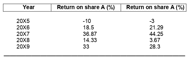
2. What is the realised average return on share B for the period 20X5 to 20X9?
A. 17.8%
B. 18.7%
C. 18.9%
D. 19.8%
3. What is the standard deviation of returns on share B?
A. 15.63%
B. 17.02%
C. 30.22%
D. 38.05%
4. What is the realised return of portfolio AB, if equal amounts are invested in each share?
A. 18.72%
B. 18.90%
C. 19.08%
D. 19.71%
5. What is the standard deviation of portfolio AB, if equal amounts are invested in each share, given the correlation of returns of A and B is 0.92?
A. 12.33%
B. 13.56%
C. 16.46%
D. 18.54%